
AI benchmarks on the stream
Same prompt, several models, measured from the transcripts: a low-poly spaceship in Blender and a low-poly island in three.js.
Why a streamer benchmarks models
Every few weeks a new AI model arrives with a chart that says it is the best. The Late Build treats those claims as content: put the models on the same job, on stream, with the same prompt, and see what actually comes out. The results here are not leaderboards. Each test was run once or twice, with a person in the loop, on one machine, so they are anecdotes with real numbers attached. What makes them useful is the method: the sessions are measured from the raw agent transcripts instead of from the models’ own summaries, and the failures are kept in.
Two tests are documented. A low-poly spaceship built in Blender through an MCP connection from a reference image, and a low-poly island written as a single three.js web page. Models in the sample include Claude Opus 5.5, Claude Opus 5, Claude Sonnet 5, GPT-6.1 Sol and GPT-6 Astra. The same experiments are written up from the product side on the Nodal site’s benchmarks page; this page tells the stream version of the story.
Test 1: the spaceship
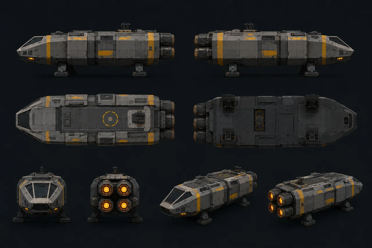
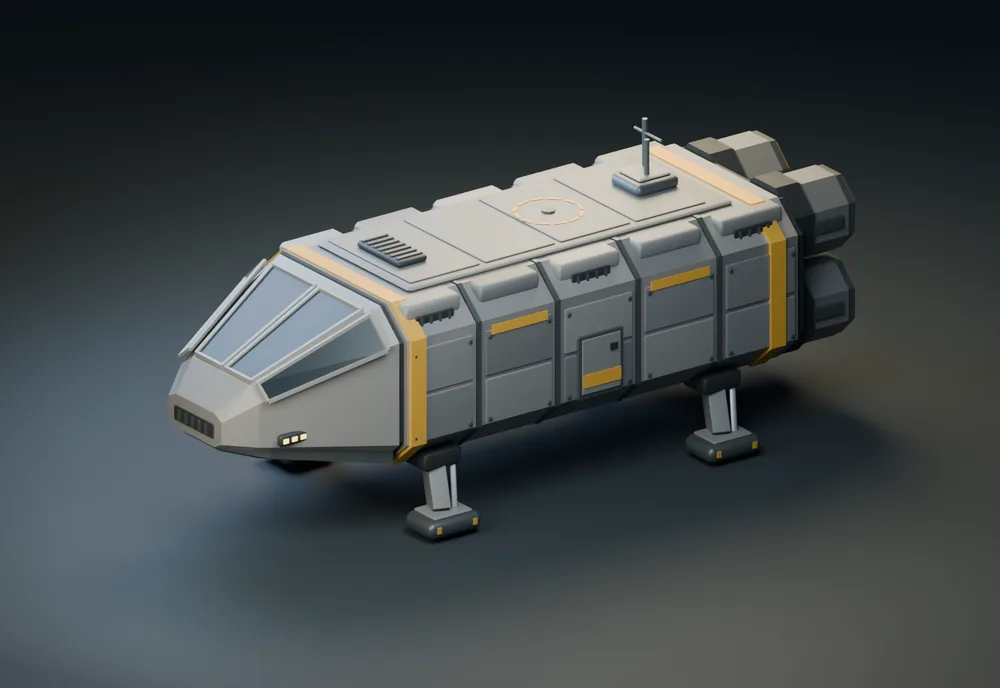
The prompt is deliberately short: “Use the Blender MCP, and model this spaceship in a low poly style,” attached to a character sheet of a boxy gray and yellow shuttle with four glowing engines and four landing legs. Each model works in a fresh Blender scene and is told not to look at other examples in the folder.
What the Claude sessions measured
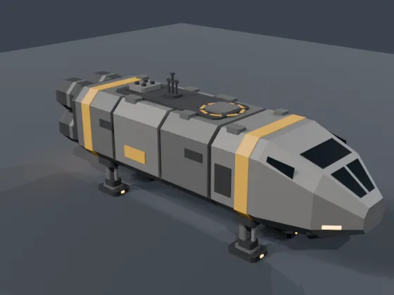
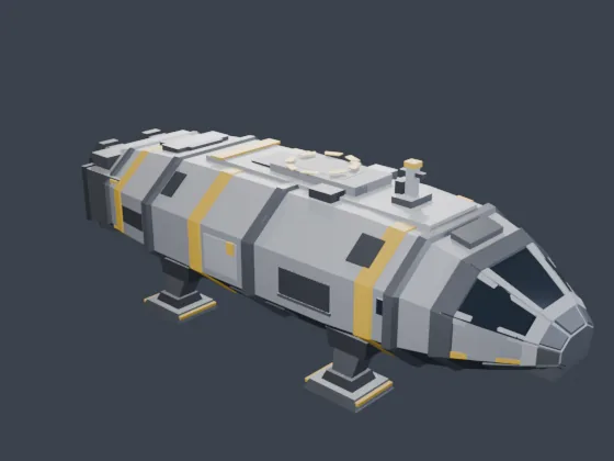
Three sessions of the same task were written up by the agents themselves with token counters, tool-call timelines and self-assessments against the reference. Two used Opus 5.5 and one used Opus 5 (a mix-up: the second session was meant to use Opus 5 but the model setting was never changed, which is why the third run exists). The comparison table is in their reports and repeated here.
| Opus 5.5, session 1 | Opus 5.5, session 2 | Opus 5, session 3 | |
|---|---|---|---|
| Tool calls | 11 | 18 | 63 |
| Code runs in Blender | 4 | 10 | 38 |
| Faces | 672 | 939 | 1,434 |
| Materials | 6 | 6 | 10 |
| Approach | One large script | Staged scripts | Render, inspect, diagnose, fix loop |
| Tokens for modeling | about 14k | about 18.4k | about 78.5k |
| Rendered images | none | none | four |
The headline is the difference in temperament. The two Opus 5.5 sessions treated the job as a one-shot generation task and used 14,000 to 18,000 tokens. The Opus 5 session treated it as a modeling loop and used about 78,500 for roughly one and a half times the geometry and a closer silhouette match, at four to five times the cost. Neither is right: it depends on whether you need a quick draft or a close match.
Lessons that transfer
- Viewport screenshots lie. They lagged behind camera changes by one or more steps, so renders written to a file and read back were both more accurate and slightly cheaper (about 150 to 190 tokens per check versus 230 to 250).
- Do not reset the scene through the connection. One helper command that reloads the default file killed the MCP server, and the build script failed with a not-connected error.
- Ask before inspecting. About 47,000 tokens went into inspecting a pre-existing scene that the user then said to ignore. One clarifying question would have been cheaper.
- Check where files are saved. One session saved to the wrong folder the first time.
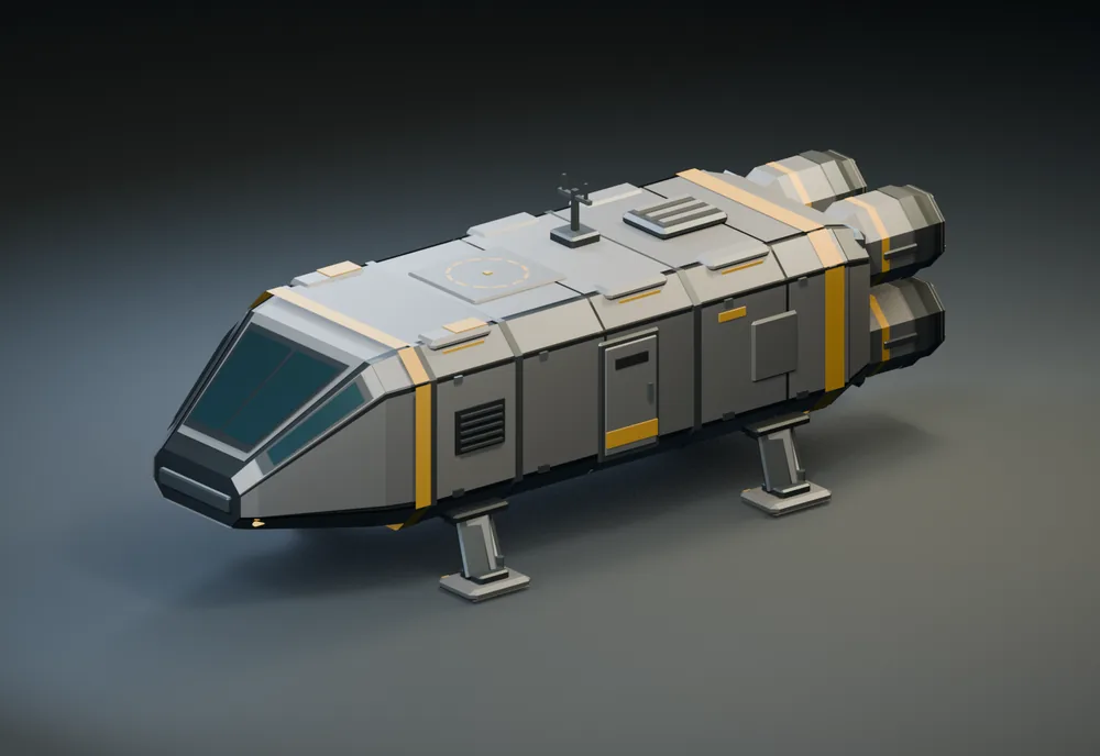
The two GPT runs came from Codex sessions that left their staged scripts and renders but no token tables, so this page shows their output without cost claims. A scoring rubric (silhouette and proportions, reference details, visual coherence, editable organization, each scored zero to five, with a triangle cap) was drafted for a planned, controlled run across five GPT models, but that run had not been done when this page was written.
Test 2: the island
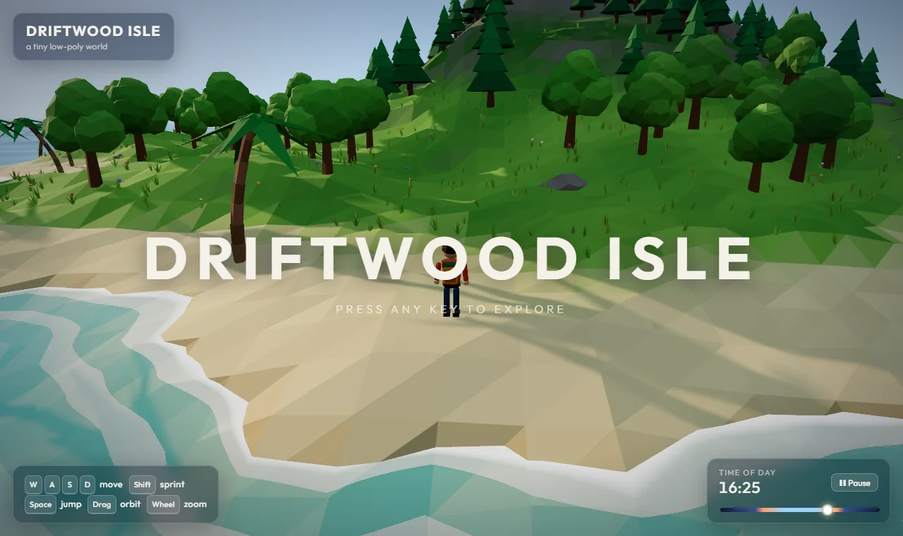
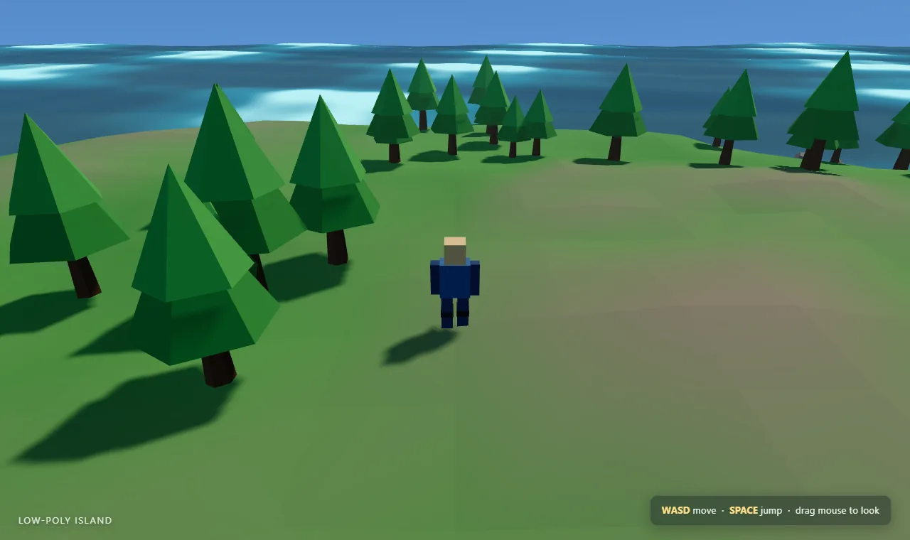
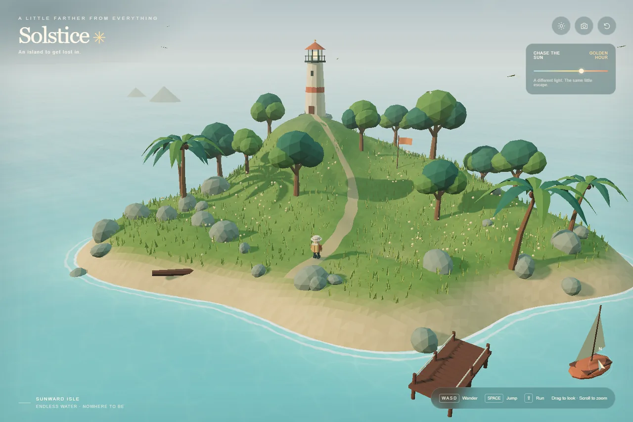
The island prompt asks for a single self-contained HTML file using three.js from a CDN that renders an interactive low-poly 3D scene: procedural island terrain, a stylized water shader, a few trees, a skybox and dynamic lighting with shadows. It must include a third-person character controlled with WASD and Space to jump, with simple camera follow. It should be visually polished, a quality showcase, with only the file as output and no explanation. A second version of the prompt asks for a high-quality non-low-poly look instead.
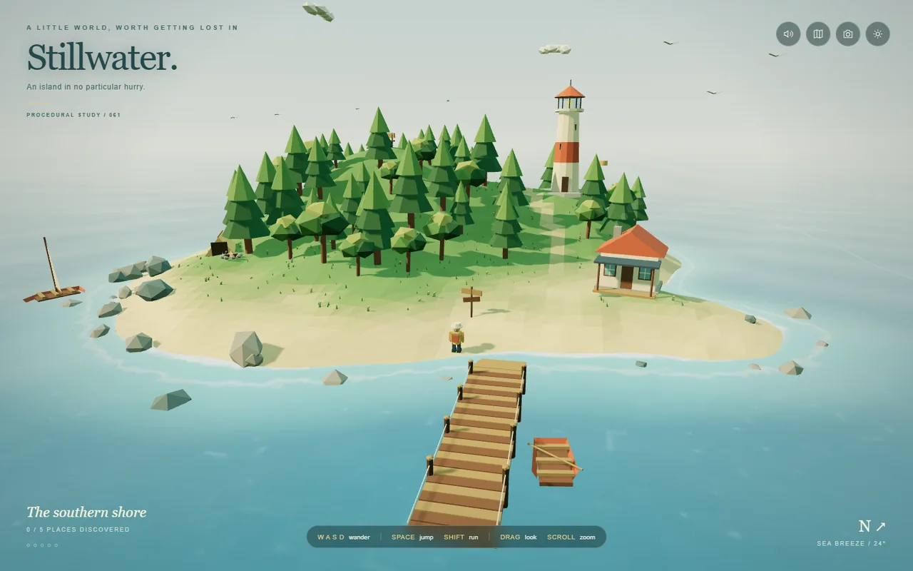
The efficiency audit
On September 23, 2026, a separate audit reconstructed three runs from the raw Claude Code session transcripts. Metrics come from per-message usage blocks, de-duplicated by message id, and costs are equivalent first-party API prices (the runs actually used a subscription). The audit’s table:
| Sonnet 5 | Opus 5.5 | Opus 5 (snapshot) | |
|---|---|---|---|
| Wall clock | 18.5 min | 9.7 min | 29.5+ min |
| API round trips | 77 | 12 | 48+ |
| Tool calls | 74 | 20 | 46+ |
| Tokens processed | 10.68 M | 1.48 M | 5.87 M |
| Equivalent API cost | $3.45 | $2.95 | $6.93 |
| File size | 23.8 KB, 692 lines | 43.2 KB, 780 lines | 45.8 KB, 1,146 lines |
| Cost per KB delivered | $0.145 | $0.068 | $0.155 |
What the audit found
- Front-loading reasoning is cheaper than iterating. Opus 5.5 spent about eight and a half minutes thinking, wrote the whole 43 KB scene in one message and then checked it with a few browser calls. Sonnet 5 wrote a file faster, then spent nine more minutes in a 74-tool-call screenshot-and-patch loop, resending about 135,000 tokens of context on every step.
- Turn count, not model tier, set the bill. Sonnet 5 has the lower per-token rate and still cost more, because each extra turn re-reads the whole context. Cache reads were 60 percent of Sonnet 5’s cost and 8 percent of Opus 5.5’s.
- Screenshot loops are expensive. Seventeen screenshots across 35 one-at-a-time browser actions each landed in a context that was re-read every turn. Opus 5 ran 89 browser actions but packed them into nine batched calls, so it paid nine re-reads instead of 89.
- Feature scan. Opus 5.5 was the only run to add a post-processing pass and particles, the “quality showcase” part of the prompt.
The caveats are in the audit too. Only Opus 5.5 ran the prompt start to finish untouched. Sonnet 5 had a pre-task benchmark turn, and Opus 5’s run was interrupted twice and asked to fix a visible bug, so its figures were a live snapshot, not a result. The page states that the feature scan measures presence and density, not visual quality, which you should judge by opening the files.
What these tests do not show
They do not rank models in general. They say nothing about long-running repository work, security or reliability across many runs. They also depend on the harness: a model that does well inside one agent tool can do worse in another, and the cost numbers depend on caching behavior that vendors change. Use them as a template for your own measurement, not as a verdict.
How to run your own
- Write the prompt on one page and freeze it. Add the output location, and say not to look at other examples.
- Use a fresh session and an empty folder for each model, with identical tools and settings. Do not run two sessions against the same Blender instance.
- Save the raw transcript. Compute tokens by category (fresh input, cache writes, cache reads, output) rather than trusting a summary.
- Judge the artifact by opening it, not by reading the model’s description. Score a few fixed criteria and blind the labels if you can.
- Record cost per accepted result, including failed attempts, and note any manual repair time separately.
- Repeat anything close or surprising. One run proves little.
The same habits appear in The vibe-coding workflow, and the usage side of cost is what AgentDashboard was built to watch. To watch these comparisons happen, see the model-comparison streams on the socials page (Days 22, 23 and 24) and the livestream page. For the Nodal angle, including how the agents in the app handle multiple models, read the Nodal benchmarks and Agent Mode pages.